Thursday 8 October 2015

Accelerated Mobile Pages

AMP : A NewAn Old Approach to Web Performance on Mobile

Like everyone else in the business, I read with interest the announcement regarding Accelerated Mobile Pages. This makes the claim:
"AMP HTML is a new way to make web pages that are optimized to load instantly on users’ mobile devices."
The "How it Works" page goes on to say:
"We began to experiment with an idea: could we develop a restricted subset of the things we’d use from HTML, that's both fast and expressive, so that documents would always load and render with reliable performance? That experiment has culminated in a promising proof of concept we call Accelerated Mobile Pages (AMP). AMP HTML is built on existing web technologies, and the documents written in it render in all modern web browsers and web views. "
There's some hyperbole here - this is not a new technique at all. Indeed, it's fair to say that the mobile revolution was kick started by a group of engineers who had near enough exactly the same insight as this "new way". Those engineers were at NTT, the product was launched by NTT DoCoMo, the subset of HTML adopted was called cHTML (compact HTML), the product was branded iMode and it was a tear-away success. IMHO, the content business model associated with iMode can also be fairly said to be the progenitor of the App Store. But that's for a different day.

cHTML?

In about 2001, there was a beautiful article in the NTT Technical Journal (English) describing why it was the cHTML was created. It's a long time ago (and I can't find the article online), but as I recall there was an oh-so-polite take down of the alternative standard for mobile web pages WAP.

My recollection is that the journal stated "we read the WAP specification and couldn't understand it, so we created something fit for purpose". So that's based off a 15 year old memory, but I think it captures the gist of what was said.

cHTML was designed with small screens, low-bandwidth, limited (four way) navigation, low device memory and low CPU in mind. Cleverly, cHTML also defined a set of icons and emoji that were guaranteed to be on the device and thus eliminated a whole range of secondary network requests.

cHTML was compact, efficient (compressed pages could often fit in one network packet), fast, worked well on tiny screens (aided by the information density of Japanese characters).

AMP?

The team that wrote AMP asked themselves
"could we develop a restricted subset of the things we’d use from HTML, that's both fast and expressive, so that documents would always load and render with reliable performance?"
Now clearly AMP is not cHTML, but there is an element of back-to-the-future here. But enough sniping, this really does solve some major problems.

I have written before about my hatred of reflow after I have scrolled a document. The AMP authors have gone-to-town on this issue and that's truly great news:

"Resources must declare their sizing up front"

This is just what the doctor ordered - in detail:
"the aspect ratio or dimensions needs to be inferable from the HTML alone. This means that after initial layout, an AMP document does not change until user action. An ad at the top of the page can’t suddenly say: “I want to be 200 pixels high instead of 50.”
There's more, but, to my mind, nothing as important as that last requirement. The 'more' includes, for example, restrictions JavaScript, CSS file size, CSS selectors, CSS transitions and animations. In addition, a whole lot of HTML tags are verboten

Final Thoughts

I'll draw one other comparison, the exorcism of Flash from mobile devices, just as it was gaining a toe-hold.

Flash (Lite) on mobile was big news in 2005-2006. Why the fall from grace? The problem was not necessarily Flash per-se, but how authors used it, particularly for ads delivered the desktop. At Phidget, I had plenty of first-hand experience of third-party Flash content where campaigns were needlessly bloated and ActionScript regularly used in tight loops that consumed 100% CPU. (One imagines this was all down to production budgets - when a piece is commissioned, I don't imagine that optimisation entered into the brief.) Whereas ad industry bodies published best practices for Flash authoring, in my experience, these were widely ignored.

Led by Apple, Flash was banned first on mobile and is now widely acknowledged to be the bad-guy on the desktop and on mobile. (Awful security does not help either.) Result: it's now into its dotage.

Another way to look at AMP is that it's a set of restrictions applied to limit the worst excesses typical practices employed by publishers who have decided to screw the experience in favour of the revenue. This is where I draw a parallel with Flash - rich campaigns with Flash were a major factor in the death of Flash as a means to create rich campaigns. Substitute the words 'ads injected by JavaScript' for 'Flash' and you have the contemporary problem that AMP seeks to solve.

AMP, like cHTML before it, has created a framework that acknowledges the user experience.

Google's backing is key here - if they prioritise AMP pages in search results, the world will be a better place as a result - SEO ranking changes will cause trickle down changes in the publishing industry.

Wednesday 16 September 2015

iOS9 and Ad-Blockers - The Problem is Reflow, Stupid!

There's a lot being written this week about iOS9 ad-blocking and page load times. Even the Sydney Morning Herald - whose six megabyte pages caused me to complain recently - is syndicating someone else's content that explains what Apple is doing.

The stories I have read focus firstly on sheer wastefulness - pointing out that the ratio of crap to content is mind blowingly large. A second theme is user tracking, which is something I also find pretty obscene (and I used to run a company that built and sold a mobile ad platform!) Finally, there is much complaint about the ads themselves - particularly interstitials.

Whereas these are all valid points, I think the real issue here is one of usability, in particular the invidious usability issue of reflow.
We've all been there. We load a page on our iPhone, we see some content displayed, we scroll down to start reading and, a moment later, the content simply vanishes off screen. This is the page reflow issue.
Asynchronous scripts insert ads into web pages. The ad injection scripts execute after page load (the Sydney Morning Herald devs would not make their users wait for 6MB to be downloaded before rendering content). Instead, the site downloads its core assets and then asynchronously loads scripts that modify the DOM, inserting video players, common content like share buttons and also ads.

The problem is that asynchronous modifications to the DOM cause the browser engine to reflow the page often altering the height of the rendered content. Clearly, vertical content heights are most likely to change on narrow width screens; on mobile that is. The issue becomes worse where multiple ads are injected into the page at uncontrolled times. Slower networks - those with limited bandwidth and/or high latencies - exacerbate the problem. Where connections to multiple hosts must be established problems are multiplied. Lower specced devices run JavaScript slowing content injection further. In summary, it's worse on mobile.

The irony in this is that web developers have had it drummed into them that asynchronous loading of assets is a good thing. Not always.


Ad injection all but guarantees an horrific user experience on mobile.

I said reflow was invidious and I mean it.

Being in the business, I understand that free is a very poor business model. When I read The Sydney Morning Herald over my Bran Flakes, I understand that the high quality content costs money to produce and that this funded at least partially through advertising. So my opinion is that advertising on the mobile web is a necessary evil and should not be blocked.

And so to iOS9 and Ad Blockers. Philosophically, I am in favour of Ads but against wholesale tracking of my movements on the web.

Ad blockers stop the reflows, stop the trackers and, given the column space devoted to this new feature, will likely lead to an uptick in usage, destroying the business model of many a web site.

Knowledgeable people say that strategically, Apple wants me to move from my browser to use Apps - including their new News offering. The analysts say that this will redirect money into their coffers instead of Google's. Apple says it's better for my privacy. The thing is though, my tool of choice for content consumption is my web browser and so I will not move to an App.

Hello then, iOS9. It's not about the Ads per se, but about the relentless, awful user experience of reflow. Although I don't want to, I will install an ad blocker.

Tuesday 15 September 2015

Huninn Mesh Part 4 - A RESTful API for Time Series Data

In this post, I will explore how we designed and built a (very?) high performance API to the Huninn Mesh server.

Beginnings

The CEO had given the requirement to "just graph it". By "it", he meant a sensor reading - temperature, pressure or humidity - and he meant a day's data. This was the point at which I walked in the door at Huninn Mesh and took over product management.

The team had already decided to build an API on the server that provided a JSON response and to use a JavaScript library on the browser to generate the graph. The API was structured as a classic HTTP GET with query parameters, something like this:

  GET /sensor?id=ae43dfc8&from=1441029600000&to=1441116000000

The result of the first sprint was a system which defaulted to plotting the prior 24 hours. That is, it used:
  • to = Date.now() and 
  • from = to - 8640000
The JSON response contained an array of approximately 172,800 arrays of raw measurements from sensors. (The system was sampling twice a second and an array of arrays was the format required for a Flot line chart).

This approach - the query design and JSON format - had the benefit of being very quick and easy to implement. Thusly, the CEO got his graph and he duly asked for two more so that temperature, pressure and humidity could be seen in stacked graphs.

The graphs were s l o w to render: running at six plus seconds. A variety of reasons conspired to make the system so slow, the number of data samples (172,800 data points / day), the fact that a query involved a Mongo DB query and then a Cassandra query, and so. In sprint two, therefore, three features were scheduled:
  1. deploy a GZIP filter in order to compress JSON response size;
  2. on-the-fly data averaging was used to reduce the number of data points to a manageable number (500 or so); and,
  3. graphs should show envelopes - maximum, average and minimum - of aggregate data.
These changes resulted in little improvement in the time to draw graph metric. This was because:
  1. the simplistic nature of the the way the query was created means that the resulting JSON was essentially never cacheable (most calls to Date.now() return a different result every millisecond and thus a different query); and,
  2. the need for on-the-fly reduction in the number of samples increased the processing time for every single query on the server by a significant amount. 
This then was the point from which a new, high performance RESTful API emerged. The decision was made to sit back, gather requirements, plan and implement a new high performance system.

It should be noted that the design work for the API was undertaken in parallel with the design for time series representation and decimation of sensor measurements - design decisions for time series representation and decimation informed the design for a RESTful API and vice versa.

Talking to Users

Whereas our first customer was our CEO, our first real users were building managers.

Huninn Mesh's first customers were the building managers of commercial real estate who loved the idea of an dense wireless network that was quickly and easily deployed, feeding a cloud based back end and providing access to a web based interface through any device.

Our first, tame, building manager asked for a tree view of sensors and a graph. In other words, something very similar to that they were used to from devices like the Trane SC.

Digging further, we found that simple graphs showing a temperature envelope were useful, but not really what they were after.


The Properties of Sampled Data

In an prior post I discussed how time-series data is organised and decimated in the Huninn Mesh server.

In summary:
  • the entire network has a fixed base sample period;
  • a device is constrained such that it must sample at a power of two times the base period;
  • data from devices is decimated by halving and stored in a Cassandra database alongside the raw measurement sample;
  • 'virtual' devices are used to provide indirection between raw samples and the outside world; and,
  • time series data from a virtual device is fixed, if an error is detected (say a calibration error), then a new virtual device is created from the raw data. 
Sampling is at a set rate which can be any power of two times the base period for the entire network.
From a raw time series, a virtual device is created and decimations calculated via a process of halving:


Halving means that decimated sample rates obey the power of two times the base period rule, just like raw measurement time series.

The trick to achieving a (very) high performance RESTful API to access these data is to design around the properties of the time series and to reflect these in a RESTful API in such a way that the workload on the server and associated databases is reduced as far as possible.

A RESTful Time Series API 

The time series API was designed to exploit the properties of predictability , immutability and decimation. The API takes the form of an HTTP GET method in one of the following variants:
  • /sensor/id/
  • /sensor/id/timezone/tz/count/sc/year/yyyy/
  • /sensor/id/timezone/tz/count/sc/year/yyyy/month/mm/
  • /sensor/id/timezone/tz/count/sc/year/yyyy/month/mm/day/dd/
  • /sensor/id/timezone/tz/count/sc/year/yyyy/month/mm/day/dd/hour/hh/
  • /sensor/id/timezone/tz/count/sc/year/yyyy/month/mm/day/dd/hour/hh/min/mm/
Where:
  • id is the virtual device id for the sensor; 
  • tz is either universal or local, where local is the local time of the sensor, not the client;
  • sc is the sample count required, of which, more in a moment;
  • yyyy is the four digit year; 
  • and so on.
The first of these API forms returns the latest measurement for the sensor. The rest should, I hope, be self explanatory.

The next sections outline how this API exploits the properties discussed earlier in order to achieve fast response times and scale.

Exploiting the Predictability of Sample Timing in HTTP

For any measurement, be it raw or decimated, the sample interval is known as is the timestamp of the last sample. Therefore, the expiry time of the resource can be calculated more or less exactly. (More or less because it is known when the sample should arrive, but this is subject to uncertainties like network latency, server load, etc.) 

Consider the following request for the latest measurement from a sensor:

  /sensor/ae43dfc8/

Assuming the sensor has a fifteen second sample rate and the last sample was seen five seconds ago, then a Cache-Control header is set thus:

  Cache-Control: max-age=10

Both the client and server can cache these responses. The workings of the server cache are discussed later. For now, it suffices to say that the server and server cache guarantee that the max-age value accurately reflects the time until the next sample is due.

The server also adds a strong Etag header to provide for the case where a measurement has expired but no new measurement has been processed by the server.

How useful is a ten second expiry time? The answer depends on whether a client or server side cache is considered. On the client, the utility is probably very small. The value becomes apparent when looking at immutability and decimation.

Exploiting the Immutability of Samples in HTTP

Every measurement, be it raw or decimated, is immutable. Put another way, a measurement never expires and the property of immutability can be exposed via HTTP's caching headers. So:
  • /sensor/ae43dfc8/timezone/utc/count/210/year/2014/ has a response that becomes immutable as soon at the year reaches 2015.
  • /sensor/ae43dfc8/timezone/utc/count/210/year/2015/month/08/ has a response that becomes immutable as soon as the date advances to 1 September 2015.
  • /sensor/ae43dfc8/timezone/utc/count/210/year/2015/month/10/day/14has a response that becomes immutable as soon as date advances to 15 October 2015.
The result of the GET request is modified thus:

  Cache-Control: max-age=31536000

Note that 31,536,000 is the number of seconds in a year and was chosen because RFC 2616 states:
To mark a response as "never expires," an origin server sends an Expires date approximately one year from the time the response is sent. HTTP/1.1 servers SHOULD NOT send Expires dates more than one year in the future.
When considering immutability of responses, the server takes into account timezone and also decimation dependencies - in other words, the expiration is correctly applied (decimation makes this more complex than one would imagine at a first glance).

What happens when a request spans a time period is best answered by discussing decimation.

Exploiting Decimation of Time-Series Samples in HTTP

Decimation is the means by which the number of samples is reduced. The sample count parameter is the means through which the user requests decimated values.

Consider a request for 200 data samples for 14th August, 2015 where the start and end of the month is defined in UTC:

  /sensor/ae43dfc8/timezone/utc/count/200/year/2015/month/08/day/14/


The server uses the sample count to select a decimated time series that provides at least as many samples as specified in the sample count for the requested period. In addition to predictability and immutability, decimation provides two major benefits:
  1. decimated values are pre-computed; and,
  2. many requests map onto one response.
Because decimations are created at a power of two times the network base period, decimation levels may not provide the exact number of samples requested, particularly at higher decimation levels.

The API implementation first checks if a decimation level maps exactly to the number of samples the given period and, if so, returns these samples. If not, the server provides an HTTP 301 (Moved Permanently) response with URL pointing at the sample count appropriate for the decimation level.

HTTP/1.1 301 Moved Permanently
Location: /sensor/ae43dfc8/timezone/utc/count/210/year/2015/month/08/day/14/
Cache-Control: max-age=31536000


Although this incurs some additional overhead, it should be noted that HTTP 301 redirects are followed transparently by XHR requests and are cacheable by the browser - for this request, the cost of a round trip to the server will be incurred once only. Of course, users of the API who know the network base period can avoid a redirect by looking up the appropriate decimations themselves.

As noted, decimated samples follow the rules of predictability and immutability, thus, as the decimation level increases, the time between samples increases and the expiry time increases. Consider two requests for a year's worth of data for a sensor where the sample count is varied:
  1. /sensor/ae43dfc8/timezone/utc/count/3375/year/2015/ 
  2. /sensor/ae43dfc8/timezone/utc/count/106/year/2015/
Given a 400ms base period for the network, request:
  1. maps to decimation level 6 where samples are updated every 00:00:25.6; and,
  2. maps to decimation level 11 where samples are updated every 00:13:39.2.
In our testing, we found that for a building management system, 200 or so samples per day proved to be more than adequate for a graph to capture the trends in temperature, pressure or humidity over a 24 hour period. For a user tracking a building, this results in a maximum of one HTTP request per sensor every 6 minutes 49.6s which represents a minuscule load on the server.

Choosing an appropriate sample count for a time series query has a dramatic effect on the likelihood of a cache hit and also server request loads


A Note on HTTP/2

Our API was designed with an eye on SPDY which became HTTP/2 during development.  By 'designed with an eye on SPDY' I mean that the design actively sought to leverage SPDY features:

  • Most particularly, the overhead of multiple HTTP requests is negligible in SPDY/HTTP 2.
  • SPDY push enables HTTP 302 (redirect) and even cache invalidations to be inserted into the browser cache.

Our server runs on Java and we chose Jetty as our servlet container as it had early support for SPDY. As it happened, this caused us some considerable pain during development as Jetty's support was immature.  As I write, we run on Jetty 9.3 (with HTTP 2) who's SPDY growing pains seem to be long behind it.

The switch from HTTP 1.1 to HTTP 2 gave us instant and fairly dramatic performance improvements with respect to throughput.  I'll talk more about these when I discuss the client side JavaScript API that sits atop of the RESTful API discussed here which will be in another post.

Strengths and Weaknesses of the Design

The obvious weakness in the API is that the end user has to make multiple requests from the server in order to assemble a time-series. This problem can rapidly become quite complex:
  • A user wishes to plot a time series spanning three entire days, all of which fall in the past, and so three separate HTTP requests must be made and the results spliced together. 
  • It is 1pm and a user wishes to plot a time series the prior 24 hour period. The user must choose whether to make two requests (as above) or 14 requests and splice them together.
  • A user wishes to plot the last two weeks of data which span a month boundary. The user can choose to make two requests (for months), or one request for the prior month and multiple requests for days for the current month, or make multiple requests for all of the days. 

The general problem of "what is the optimum sequence of requests to fulfil an end user's data requirement?" gets harder if the hour / minute API is used.

More subtly, a (power) user has to be not only smart but also consistent about which requests to make if they wish to maximise the chance of a cache hit and therefore deliver the best interactive performance to the end user.

Finally - and perhaps most importantly - splicing the results from multiple requests that might span multiple time spans and perhaps also have missing data is just painful.

The API is: RESTful; individual requests are fulfilled very quickly; a great match for HTTP/2, but that does not mean it is easier than the old-school API we started with: it isn't.

These are real issues and, at Hunnin Mesh, we immediately ran up against them when dogfooding our UI for building managers. Since I designed the API, I knew from the outset that a JavaScript wrapper would be needed that exposes a higher level API - one that supports date range requests. That API went through two major versions - the second of which was a major undertaking - and I intend to write about it in my next post.


Summary

This architectural approach can be summarised as follows:

  • Immutable time series means cacheable HTTP responses which, in turn, means that Cassandra queries stopped being a bottleneck. 
  • HTTP responses are cached at the server and may be cached at the client.
  • Responses can be pre-computed and, therefore, the server cache can be primed.
  • Deployment on an HTTP/2 server (Jetty) meant that the network overhead of many HTTP requests is immaterial to performance. 
  • The job of the server then is typically reduced to authentication and serving of static responses from a cache.

We started with a traditional query based API which delivered page load for three graphs (three requests) in approximately six seconds.

A measure of our success is that with an empty browser cache, in six seconds, we were able to increase the number of objects graphed from three to six hundred. 

Moreover, irrespective of whether the browser was able to displaying a year's data, a month's, a day's or an hour's, the time to render was a nearly constant.

I'll write another post musing about the services provided by this JavaScript API at when I get the chance...

Friday 28 August 2015

Huninn Mesh Part 3 - Organisation of Time Series Data

In my previous two posts about Hunnin Mesh, I discussed the nature of the Huninn Mesh network and the architecture, abstractions and constraints of the Huninn Mesh server.

In this post, I will go into more detail about the organisation time series data in the Hunnin Mesh server and will illustrate how the system is designed to achieve high throughput in terms of both measurement ingestion rates and also access to data by end users through a RESTful API.

The Huninn Mesh Network

Huninn Mesh manufactures wireless sensors that measure temperature, pressure, humidity and so on. The sensors are arranged into a mesh network. That is, a network where one sensor 'node' can pass information to another mesh node, and so on, until a gateway device is reached. The gateway then passes measurements to a server that resides in the cloud.

Huninn Mesh is a mesh network of sensor nodes (blue) which communicate using the Huninn Mesh protocol (orange lines) through a gateway (purple) to a server in the cloud (black line).
A Huninn Mesh network is:
  • software defined (routing of messages is under the control of a server in the cloud; 
  • able to efficiently handle large number of hops between network nodes; 
  • resilient (it is able to recover from the failure of a node); and,
  • quiescent for most of the time (nodes are quite literally off line, relying on schedule specified by the server to perform allocated tasks).
A Huninn Mesh sensor is:
  • compact (10cm by 10cm by 1.5cm);
  • typically measures two to three parameters - temperature, pressure and humidity being the most common;
  • battery powered; and,
  • designed to provide a realistic battery lifetime when deployed in the field of five years and is sampling at 15 second intervals.
A Huninn Mesh server is responsible for:
  • managing the mesh (creating and updating the software defined network);
  • managing sensors;
  • ingesting data from sensors;
  • storing data in a time series database; and
  • exposing an API through which the data can be queried.
The characteristics of battery powered sensor nodes coupled with a software defined mesh network topography mean that large numbers of Huninn Mesh sensors can be deployed by non technical people in a very short time and, therefore, at a low cost.  The server architecture leverages the power of cloud based computing and mass storage, again, at a low cost.

Using the Data Stream

To date, Huninn Mesh networks have been installed in office buildings in order to provide the measurement base on which building managers can optimise building comfort and energy usage.

Using a real world example of a fifty floor building in New York, over two hundred sensors were deployed, each of which samples temperature, pressure and humidity at roughly fifteen second intervals. Thus, the server receives approximately 2,400 measurements per minute from this network (this measurement ingestion rate of 40 transactions per second is roughly 1/5,000th the capacity of a single server - we regularly test at 5,000 tx/sec).

Different users have different requirements of this data set. Interviews with building managers tell us that they require:
  • proactive hot/cold/comfort alerts;
  • reactive hot/cold reports;
  • suite/floor/building comfort state visualisation;
  • seasonal heat/cool crossover planning; 
  • plant equipment response monitoring;
  • comparative visualisation of different buildings; 
  • ad-hoc data query for offline analysis (in Excel);
  • and so on.
From the above, it should be clear that:
  • a building manager requires aggregate data sets that represent multiple sensors; and,
  • in most cases, measurements made at fifteen second intervals provide far more information than the requirement demands (a manager does not require 5,760 data points in order to ascertain the trend in ambient air temperature of a building's lobby over a 24 hour period).
At Hunnin Mesh, the question of how to make our data set fit for these many purposes occupied us for some time. The solution was decimation and the creation of Computational Devices and that's what the remainder of this post is about.

Time Series Data Set Decimation

Decimation refers to the (extreme) reduction of the number of samples in a data set (as opposed to one-tenth as implied by deci). Decimation in signal processing is well understood. I'll explain how we use the technique in the Huninn Mesh system.

A Huninn Mesh sensor samples at a set rate and this rate must be a power of two times a base period defined for the entire network.  In this illustration, the sample rate is fifteen seconds.

Samples are obtained at a regular interval.
Our problem is that the number of samples is (often) too large and, therefore, the data set needs to be down-sampled. The Huninn Mesh server does this via decimation - it takes a pair of measurements and calculates a new value from them.

A pair of samples taken at 15 second intervals (black) is used to create a new sample (blue) which contains the maximum, minimum and average of the two raw measurements and has a sample rate of half that of the original pair and with a timestamp half way between the timestamps of the two measurements.
The calculation of the aggregate value depends upon the type of 'thing' being down-sampled. In the case of a simple scalar value like a temperature measurement, the maximum, minimum and average of the two samples is calculated. This aggregate sample is stored in a Cassandra database in addition to the raw data series.

Decimation is also applied to values created by the decimation process. With four samples, the system is able to decimate a pair of decimated values (using a slightly different algorithm).

Decimation (purple) of a pair of decimated values (blue) which are calculated from the raw time series samples (black).
And with eight samples, a third decimation level can be created and so on:

Three 'levels' of decimation (orange) require 2^3 = 8 raw time series samples and each individual derived value and is representative of the entire two minute period.
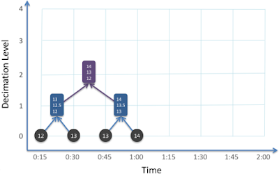
The calculation of decimated values proceeds as shown in the following animation.
The calculation of aggregate values representing different decimation levels occurs when the full sample set for the aggregation is available.
A Huninn Mesh server is typically configured decimate over 24 levels from the base period of the network with the first level aggregating over 2 samples, the second 4, the third 8, to the 24th which aggregates 16,777,216 base period samples. In fact, for any given decimation level, only the pair of values from the previous level are required to perform the decimation meaning that the process is computationally efficient regardless of the decimation level and requires a small working set in memory.

The raw time series measurements and all decimated data products for every sensor are stored in a Cassandra database. The API to query this information will be discussed in a follow up post.

Recall from an earlier post that every Huninn Mesh device in a network has a sample rate that is a power of two of a base period that is constant for the entire network. Therefore, decimation intervals exactly match sample intervals allowed for sensors.

A fixed base period and the rule that sensors must sample at a rate that is a power of two times the base period provides a guarantee higher order decimations will be available. Samples are all aligned in time. In fact, neither samples nor the decimation time window are aligned. Instead, the actual time that a measurement is made depends upon the optimum network configuration. The system only guarantees that measurements will be made at the required interval.

If the base period were set at 400ms, the decimations would proceed as follows:

Decimation
Level
Samples
Aggregated
Interval
(ms)
Time Span
(D H:M:S.ms)
1 2 800 00:00:00.800
2 4 1,600 00:00:01.600
3 8 3,200 00:00:03.200
4 16 6,400 00:00:06.400
5 32 12,800 00:00:12.800
6 64 25,600 00:00:25.600
7 128 51,200 00:00:51.200
8 256 102,400 00:01:42.400
9 512 204,800 00:03:24.800
10 1,024 409,600 00:06:49.600
11 2,048 819,200 00:13:39.200
12 4,096 1,638,400 00:27:18.400
13 8,192 3,276,800 00:54:36.800
14 16,384 6,553,600 01:49:13.600
15 32,768 13,107,200 03:38:27.200
16 65,536 26,214,400 07:16:54.400
17 131,072 52,428,800 14:33:48.800
18 262,144 104,857,600 1 05:07:37.600
19 524,288 209,715,200 2 10:15:15.200
20 1,048,576 419,430,400 4 20:30:30.400
21 2,097,152 838,860,800 9 17:01:00.800
22 4,194,304 1,677,721,600 19 10:02:01.600
23 8,388,608 3,355,443,200 38 20:04:03.200
24 16,777,216 6,710,886,400 77 16:08:06.400

The Time Span column gives the number of days, hours, minutes, seconds and milliseconds represented by a single decimated value.

Note that earlier, I wrote that the sample period was 'roughly' fifteen seconds. In fact, the network had a base period of 400ms and so the sample period was 12.8 seconds.

The next section provides more detail about the properties of of time periods including alignment with human recognisable intervals.

Properties of the Time Series

At the risk of stating the obvious, the first property of note is that for any given sensor at any moment, the length of time until the next measurement is available is always known irrespective of whether the measurement is raw data or an aggregate decimated value (this property is very useful and its use will be discussed in my next post about the Huninn Mesh RESTful API for sensor data).

The second property arises as a result of the network having a constant base sample period: device sample rates and decimated sample rates align across a network. Individual devices are constrained such that they must only sample at a rate that is a multiple of a power of two of the base rate. For example, on a network with a 400ms base period, one device may sample every 102,400ms and another 12,800ms and another at 800ms: through decimation, data for all of these devices can be accessed at sample rates that are known a-priori.

The third property is that time spans for decimation levels do not map exactly to any human recognisable span: no decimation level that maps exactly to an minute, hour, a day, etc.

This last property means that there will always be an error in when estimating values for one of these 'human' periods. For example, what if the daily average for a temperature sensor is required by a building manager? Since there is no decimation that maps exactly to a day, the trick to using these data products is to select a decimation level that provides the smallest number of samples (with an acceptable error for the period under investigation) and then to calculate the mean from this small set.

Where a single sample is required to summarise a day, the following decimations might be considered:
  • Decimation level 18 provides a single sample that spans one day, five hours, seven minutes, 37 seconds and 600 milliseconds. This is unlikely to be of use because it spans more than a day and individual samples do not align on date boundaries. 
  • Decimation level 6 samples at 25,600ms which divides exactly into 86,400,000 (the number of milliseconds in a day). At this decimation level, there are 3,375 samples per day which would have to be averaged in order to calculate the required data product. This represents 1/64 of the raw data volume but the maximum error of 25.6 seconds may be overkill for the requirement.
  • Decimation level 10 creates a sample every 409,600ms (about every six minutes and fifty seconds), each sample aggregates over 1,024 raw measurements, returns 210 measurements per day that must be averaged to provide the end result and has a sample error of 6 minutes 24 seconds.
  • Decimation level 14 creates a sample every 6,553,600ms (about every one hour and 39 minutes), each sample aggregates over 16,384 raw measurement, returns 13 measurements per day that must be averaged to provide the end result and has a sample error of 20 minutes and 3 seconds. 
In the web based API provided by Huninn Mesh for building managers, we chose decimation level 10 which returns 210 samples that then have to be averaged to provide the mean for the day.  This decimation level was chosen because the sample time error was small (a maximum of six minutes and ten seconds) and this number of samples also accurately catches trends in temperature / pressure / humidity in a building and so the data set is also useful for graphing.

In this discussion, the sample error refers to that part of a day that is under sampled when using the given decimation level (a user could also choose to over sample in order to fully bracket the required time span).

In summary, the properties of the raw time series and decimated data products mean that the system does not provide answers to questions like "what is the average temperature for the day for sensor X". Instead, the system creates and stores multiple data products that can be rapidly queried and post processed by the user to arrive at an answer.

Computational Devices

Up until this point, discussion has been concerned with measurements from physical sensor devices - little boxes that measure temperature, pressure, humidity and so on. One of the use cases presented for the instrumented building discussed earlier was what is the average, maximum and minimum temperature for the entire building, that is, a measurement that represents a number of other measurements.

Computational devices are a special class of virtual device, implemented in software, that sample measurements from other devices (both real and computational) and emit a sample of their own.

For example, an Aggregating Computational Device may be created that takes as its input all of the devices that produce an aggregate temperate value for every floor in a given building. The devices for the floor are themselves computational devices that take as their input all of the raw temperature sensors on the given floor.

Nine 'real' devices (blue) measure temperature on three different floors and are used as inputs to three Computational Devices (tc[1]... tc[3]), each of which aggregates over the temperature for an entire floor and are used as inputs to a single computational device (tc[b]) that aggregates over the temperature for the entire building (right). 
In the diagram, above, the arrows between devices show the logical flow of data, arrows should be interpreted as meaning 'provides an input to'.

Just like every other device, Computational Devices sample - they are scheduled at a set rate. They do not wait for events from dependent devices and, for this reason, circularities can be accommodated - a Computational Device can take as input its own state. Sampling theory says that a Computational Device should sample at twice the frequency of the underlying signal: twice as often as the smallest rate of any of the 'real' sensors.

To date, two types of Computational Device have been created:
  1. Aggregating Computational Devices sample either real devices or other Aggregating Computational Devices and emit the average, maximum, minimum, average-maximum and average minimum; and,
  2. Alerting Computational Devices sample either real devices or other aggregating computational devices and emit either an enumerated value (e.g. hot, cold, normal).
We have a range of other devices in the works, for example, ASHRAE comfort devices for summer. Ultimately, Huninn Mesh intends to release a public API whereby users can plug their own computational devices into the system.

The output from a Computational Device is subject to decimation, just like any other device. Time series data from computational devices is stored in a Cassandra database, just like any other data. A computational device is, however, able to specify its own format for storage in the database and its representation through the Huninn Mesh RESTful API.

Programatically, Computational Devices are described by a simple programming interface in Java. It is a straightforward matter for a competent software developer to implement new types of device - for example, a simple extension to the Aggregating Computational Device is one which weights its inputs.

Time Series Data a Device is Immutable

A final rule worth touching upon is that the raw time series and the associated decimated data set for a device is immutable: once created, it cannot be altered. Data is written once to Cassandra and read many times.

What happens then if there is an error? for example, a device is deployed for some time before it comes to light that the calibration is incorrect? (As it happens, this was our most common error during development.)

The system is architected so that sensors do not perform conversion or calibration in the network. Instead, the raw bitfield is always passed to the server which:
  1. stores the raw bitfield in Cassandra against the ID of the Real Device; and,
  2. converts, calibrates and decimates measurements and stores these against a Virtual Device ID in Cassandra.
Calibration and conversion is a property of a Virtual Device's specification. If the calibration is changed retrospectively, a new Virtual Device is created for the affected Real Device and historical data replayed to create a new time series.

Put another way, fixups are not allowed - time series data really is immutable. This is not to say that corrections cannot be made, they can. A new Virtual Device is created and the raw data stream is replayed, recreating a new, correct data set. The same is then done for all downstream Computational Devices including their descendant Computational Devices.

This begs one question: if Virtual Devices are subject to change, how does an end user discover what device represents what property - which device can tell me the average temperature for building A?

The answer to this question is in a device discovery API and this will be discussed in my next post about the Huninn Mesh RESTful API.

It's About Scale

Fixing the network's base sample period, the power of two times base period rule, decimation, computational devices, device virtualisation, and immutability are all features that have been honed with one need in mind: performance at scale.

Consider that:
  • For any decimation level, the arrival time of the next sample is known in advance, or, put another way, the expiry time of the current measurement is precisely known.
  • Reduction of the time series through decimation has a low computational overhead and can dramatically reduce the amount of data required to answer any given query. 
  • Immutability of any measurement point at any level of decimation for a virtual device means that the sample never expires: it can be safely cached outside of the system forever.
  • Indirection through device virtualisation introduces the need for a discovery API, the results of which are the only part of the system subject to change.
In my next post, I will discuss how all of this comes together in the Huninn Mesh RESTful API to deliver a system with very low query latency times across very large numbers of sensors and multiple orders of magnitude of time ranges.

Thursday 13 August 2015

Did I Click That? or What's up with the Browser User Experience on Slow Network Connections

My Network is Slow

For some reason, right now, there is an awful lot of time between my clicking on a link in a web page and any content displaying in my browser. Things are wrong, things are going wrong: it seems that my ADSL network is at a crawl, that DNS queries are incredibly slow, and overall round trip latency even to a server just across the city is awful.

How wrong? Well, I'm writing from Sydney and browsing the Sydney Morning Herald home page (251 HTTP requests, 6,106KB) and it is taking 8 seconds to reach a page load event. Following a link from the home page (Commonwealth Bank customers say double charges not refunded), I see (an incredible) 340 requests and a further 10,467KB downloaded - with a 6 second delay until I see content.

The purpose of this missive is not to complain about the absurd weight of the two pages cited, but to discuss the user experience during the (seeming interminable) wait for content. Since I use Firefox as my default browser, I'll (mostly) confine my comments to that browser, although my comments may be applicable to other browsers - mobile and desktop.

Did I Click That?

As noted, what's happening right now when I click on a link is, well, nothing much. I can't do much about my network, but the issue of nothing much happening at all might be improved upon.

Let me explain by walking through my actions and Firefox's response when viewing articles on the SMH website:
  1. I move my mouse over an article link;
  2. my mouse cursor changes, the anchor tag for the link is underlined as I hover over it and the title specified in the anchor is shown (all from HTML/CSS/JS);
  3. the URL associated with the link is shown in a small, animated, floating status bar overlay in the bottom left of the browser window;
  4. I click my mouse to follow the link - nothing changes between the mouse down and mouse up (again, HTML/CSS - i.e., no CSS :active selector on the SMH website);
  5. as I release the mouse button the link turned grey (CSS :visited selector at a guess);
  6. the tab in my browser changes from showing the page title to displaying an animated 'throbber' alongside the word "Connecting" and the status bar changes according to page load state - for example, "Waiting for smh.com.au", "Read smh.com.au" and so on;
  7. a few seconds later, the tab changes, showing the title of the new page as the browser receives and parses the HTML head element from the server (like I said, things are wrong...); and finally,
  8. some time afterwards, the page renders and the 'throbber' icon is replaced by a favicon for the site.
Chrome does something different, but you have to be observant to note that it shows the domain name (www.smh.com.au) when it is in the 'connecting' state and it also shows various 'processing' messages in its status bar during page load.   On closer inspection, Firefox does almost exactly the same thing.

Here's a screenshot of Firefox on a Mac showing a page load in progress, with the tab-bar 'throbber' and status bar both highlighted.
Firefox's loading 'throbber' and status bar during a page load.

Given my slow connection, my experience of clicking a link is poor - it's difficult to understand what's happening.


Why so? My eye and therefore my focus is directed to the link that I clicked, not the 'throbber' in the tab bar and not on the status bar.

Given a slow connection, in order to verify that I have actually clicked on a link, my eye has to scan up to the top of the page and then across in order to locate the tab containing the throbber. Alternatively, my eye can scan to the bottom left of the page. Either way, on my slow connection it is not immediately apparent what the browser is up to, leaving me in a state of cognitive dissonance - I clicked that link, didn't I?

Experimenting on Children

As I write this, I have been careful to control my own behaviour. In particular, I have made sure that I click on links once and only once. That's because I know that, just like a pedestrian crossing where pressing the button multiple times does not make the lights change faster, the page won't load any faster if I click the link lots of times. I tell my kids this, but they press the button at the crossing fifty times and a simple experiment this morning reveals that they do exactly the same thing when faced with links that do not result in near instantaneous page loads.

Unlike pedestrian crossings, clicking the link on the web page multiple times does change the outcome. A quick look in the developer tools (Chrome) shows that when the littlies repeatedly click on the same link, outstanding network requests are cancelled.

In an HTTP/1.1 world, this is bad news. I mean really, really bad news for performance. This is because a cancelled request results in a torn down connection (TCP close and all that). Only to be re-established and the same HTTP request re-sent. (In the interests of balance I should add that, networks being what they are, this strategy sometimes works.) I should also add that in an HTTP/2 world, the cost is nothing like as great but it still exists, particularly in the case of network that's just plain slow.

A Modest Proposal

At the risk of stating the obvious, sites should do what they can with HTML/CSS/JS available to them to provide appropriate cues to the user regarding followed links and progress. That's not what this proposal addresses, however. I am making a suggestion about what the browser might do during a page load and is thus outside of the realm of normal HTML/CSS/JS.

From a product perspective, I believe that changing the experience of page loads can improve the user's understanding of what just happened and, by so doing, reduce the number of false reloads which, in turn, might actually improve performance on slow networks.

As noted earlier, the state of the art is a throbber in the tab bar and a part-time status bar. The key change I suggest is to (drastically) change the way that page loading state is conveyed. If we accept that the user expects something to happen immediately on clicking a link, then it is reasonable to use the entire browser window's drawing area to convey feedback about the page load operation. Users are accustomed to modal progress spinners in their mobile apps and I am proposing something similar, but writ large:

It's clear that a link was clicked, a page is loading, and the most common options are clearly accessible to the user.

Looking past the fact that I just threw this together using Gimp and Powerpoint, there are a number of product requirements here:
  1. The act of clicking on a link that navigates away from the current page should result in immediate unequivocal feedback irrespective of page design, the speed of the network, remote server, etc. (More on 'immediate' in moment.)
  2. Information from the anchor URL and title in the followed link should be used to provide feedback about what page is being loaded.
  3. Navigation away from a page is immediate and so all other links on the page should be disabled.
  4. The user should be provided with a simple means to cancel the page load operation and go back to the prior page.
  5. Because sometimes networks will be networks, a means to cancel a slow request and restart it should be provided. 
Arguably the browser already covers off on points 1, 2, 4 and 5.  Therefore, I am only arguing for a change in how this information is presented.

In practice, this might work as follows:
  • The user clicks a link to navigate away from the current page.
  • An interstitial loading page is inserted into the tab comprised of:
    • a background image created from a screenshot of the page being unloaded, with a Gaussian filter applied, is used to indicate that links cannot be followed during page-load. (I chose a Gaussian filter because, hey, why not?);
    • an animated throbber echoes that in the tab bar;
    • the title of the page being loaded (from the anchor element) allows the user to intervene early in the case where the wrong link is clicked;
    • the domain name of the server being contacted is prominent and may assist the user in an early bail-out;
    • a button that provides the user with a means to go back to the prior page; and,
    • a button that allows the user to reload the page.
  • Immediately on receipt of the head element for the new page, the link title is updated in the interstitial and tab bar (so you know you're being rickrolled, just before you really are).
  • The interstitial page is removed and replaced with the new page contents as soon as enough content has been retrieved from the network.  They key requirement here is to avoid replacing the interstitial with a blank page during slow loads.  I'm aware of how hard this may be to implement, what with CSS + JS but see no harm in asking.
In order to cater for fast page loads, the creation of the interstitial might be staggered. On navigation to a new page:
  • Links on the existing page are immediately disabled.
  • The interstitial is immediately created containing a blurred copy of the prior page but with the other interstitial UI elements hidden.
  • Some time later - say 500ms - the throbber, text and button elements are made visible in the interstitial.
Whatever the new UI does, it should not degrade the user experience of fast loads, that is.

At this point, my imagination is galloping off - timing of the creation of the interstitial might be varied depending on whether a connection to the host is already open, or whether the link is to the same domain as the page being unloaded. I use a range of apps such as JIRA where one page looks very much like another. In this case, the bluring and redrawing of near identical pages during navigation might be distracting. Again, timing is key. Animation may be useful. I should stop - my point is that immediate might mean in the blink of an eye.  In summary, I think that this idea will be useless if the timing of the presentation of the interstitial is wrong.

HTTP GET requests require no further discussion. Since POST requests are not idempotent, they must work as they currently do, that is, if the user retries a request, they must be warned that information will be submitted twice.

For the avoidance of doubt, I believe this might work for normal links but not for JavaScript.

Summary

In the world of mobile apps, it is common to provide a modal 'spinner' that is displayed in response to a user action to signify that the app is busy, for example whilst waiting for an operation like a network request to complete.  This idea expands upon this.

Utilising the whole of the browser window in order to provide feedback during slow page loads may provide an improved user experience and possibly even lead to modest improvements in load time outcomes.  I reason that the idea is equally applicable to mobile as it is for desktop browsers.